
Yes, truck driving, one of the most essential industries in the US, as it rakes in 700 billion and accounts for 5% of the GDP. So, it must be important to optimize this important sector of America. Which drivers are high performing? Which drivers are not? Of course, I asked myself and my team these thought-provoking questions when we were trying to understand how data science works.
There tends to be a high turnover rate in the trucking industry, there’s low pay and forced dispatching. To tackle this, we decided to make a model for NEXT Trucking, a California based company founded in 2015, to help make their drivers more appreciated. By working with real data and creating an intuitive model, we obtained a better understanding of the base of a typical data science lifecycle.
Data Preprocessing:
Generating the Label:
What constitutes a high performing driver? A good answer would be simply how many loads one has delivered, and drivers that are active. So, a high performing driver would be one that delivers a lot of loads and has performed recently. We took the 75% percentile of drivers in the variable “total_loads” and the 25% percentile of drivers in the variable “most_recent_load_date”. This allowed us to label the select drivers in this group as high performing.
This approach brings up the problem of having an uneven class label distribution. It only labelled 1% of the dataset as high performing. To tackle this, we need to undersample and oversample the different groups.
Imputation:
To undersample the majority class(the 1% of high performing drivers) we would need to reduce the number of data observations. We can do this using a simple RandomUnderSampler().
To oversample the minority class of high-performing drivers, we used the SMOTE algorithm. It works by selecting similar data samples in terms of the features, and connects them with a line. It then creates new data samples on that line, giving us the artificial data that we needed.
Two features that we also decided to change were in relation to where a driver was from. “home_base_state” is the state that a driver is from, since the majority of drivers were from California and it has a similar distribution to the population we just replaced all the null values with CA. Next, “home_base_city” had some missing values, so we just replaced those with a random city in California.
Aggregated Features:
The original dataset contained daily job entries performed by drivers, but the goal was to classify the drivers themselves. To achieve this, we grouped each unique driver by their id, and aggregated features were computed to summarize their past performance. For example, features like the number of jobs per weekday, month, and year were created to capture the seasonality and sparsity of their work activity. We could then collapse the dataset to have each row represent a unique driver with their aggregated characteristics.
Encoding/Transformation for new features:
We found that there were two variables in the dataset that weren’t very significant on their own, but are more appropriate when combined. “port_qualified” determines if a driver can perform jobs in port terminals, and “interested_in_drayage” are drivers that are interested in performing drayage routes. Since port terminals are typically drayage services, we decided to combine the two using a logical AND.
Next, we wanted a feature that represents the time it takes for a carrier to be approved after signing up for the NEXT platform. It would be transformed into an ordinal variable with three categories: • 0: Approved between 1 and 31 days. • 1: Approved between 31 and 91 days. • 2: Approved after more than 91 days (or not yet approved). This transformation categorizes the approval time into meaningful groups that capture different stages or durations of the approval process.
We also wanted a feature that captures the seasonal availability of each driver. We decided to use the “load_day” and represent each month (Jan-Dec) as a separate feature. The value of each feature represents the number of jobs a driver completed in that particular month. This transformation helps capture the patterns or variations in driver activity across different months and accounts for the seasonality in the data. The “month” feature is then standard-scaled, which typically involves normalizing the values to a common scale to prevent any bias during model training.
Data cleaning:
For the variable that associated the number of trucks with a driver, there would sometimes be a 0 value. We decided to drop these observations as it made no sense for there to be no trucks with a driver that performed. Also, the variable that represented the lanes a driver preferred only had 194 non-null features, so that feature was dropped. Many other features that had no significance to a driver’s performance were dropped, such as the date of the loads serviced or the carrier company name.
Feature Processing:
The dataset contained both categorical and numerical features that needed to be processed before using them in the models. Categorical features required encoding techniques like one-hot encoding, while numerical features needed scaling to bring them to a similar range.
The following table summarizes how handled each of the original data features:
| Feature Name | How We Handled It | Explanation |
|---|---|---|
| dt | Dropped | Short for date |
| weekday | Expanded into 7 features (Mon. - Fri.), then standard-scaled | Day of the week (Monday for example) |
| year | Expanded into 6 features (2015-2021), then standard-scaled | Year value parsed from field dt |
| id_driver | Dropped (trivializes label prediction) | Driver ID |
| id_carrier_number | One-hot encoded with drivers who are also owners received value “independent” | Carrier number. For carrier type equals to fleet, one carrier can have multiple drivers; while for carrier type equals to Owner Operator, one carrier has one and only one id_driver. |
| dim_carrier_type | Dropped in favor of id_carrier_number | Two types of carriers, one is Fleet and the other is Owner Operator. For Fleet, it can be a small company with multiple truckers but for Owner Operator, it usually only has one trucker. |
| dim_carrier_company_name | Dropped in favor of dim_carrier_type | Carrier company name |
| home_base_city | One-hot encode | The home base city the driver claimed |
| home_base_state | One-hot encode | The home base state the driver claimed |
| carrier_trucks | One-hot encode truck types | Type of the trucks |
| num_trucks | Standard Scaling | # of trucks associated with this carrier |
| interested_in_drayage | Binary encoded | If a carrier reported himself or her interested in providing drayage services, this field becomes true |
| port_qualified | Binary encoded | This field becomes true if a carrier reported him or herself as port qualified |
| signup_source | Binary encoded | Can be mobile or other as the value |
| ts_signup | Dropped in favor of time_to_approval | Signup timestamp |
| ts_first_approved | Dropped in favor of time_to_approval | The timestamp if a carrier was first approved. If null that means Next Trucking has not approved this driver yet. |
| days_signup_to_approval | Dropped in favor of time_to_approval | If a carrier was approved, this field will be a non-null value which calculates the date from first signup till approval date |
| driver_with_twic | Binary encoded | If a driver has TWIC insurance then this field will be true |
| dim_preferred_lanes | Dropped | The driver can specify which lanes (preferred routes) he’d like to take |
| first_load_date | Converted to the number of days ago (from today) and then standard-scaled | The date the driver serviced his first load |
| most_recent_load_date | Dropped (trivializes label prediction) | The date the driver serviced his most recent load |
| load_day | Dropped | The date of the loads serviced |
| loads | Dropped | # of the loads a driver serviced |
| marketplace_loads_otr | Standard Scaling | An OTR (over-the-road) type of the loads covered by driver from marketplace (our app) |
| marketplace_loads_atlas | Standard Scaling | An drayage (ATLAS is our in-house solution that hosts drayage jobs) type of the loads covered by driver from marketplace (our app) |
| marketplace_loads | Standard Scaling | The sum of marketplace_otr and marketplace_atlas |
| brokerage_loads_otr | Standard Scaling | An OTR (over-the-road) type of the loads covered by a driver assigned by brokers which is a more traditional way and we have less control on. |
| brokerage_loads_atlas | Standard Scaling | An drayage (ATLAS is our in-house solution that hosts drayage jobs) type of the loads covered by a driver assigned by brokers which is a more traditional way and we have less control on. |
| brokerage_loads | Standard Scaling | The sum of brokerage_loads_otr and brokerage_loads_atlas |
| total_loads | Dropped (trivializes label prediction) | The sum of brokerage_loads and marketplace_loads |
Data Exploration and Analysis (EDA)
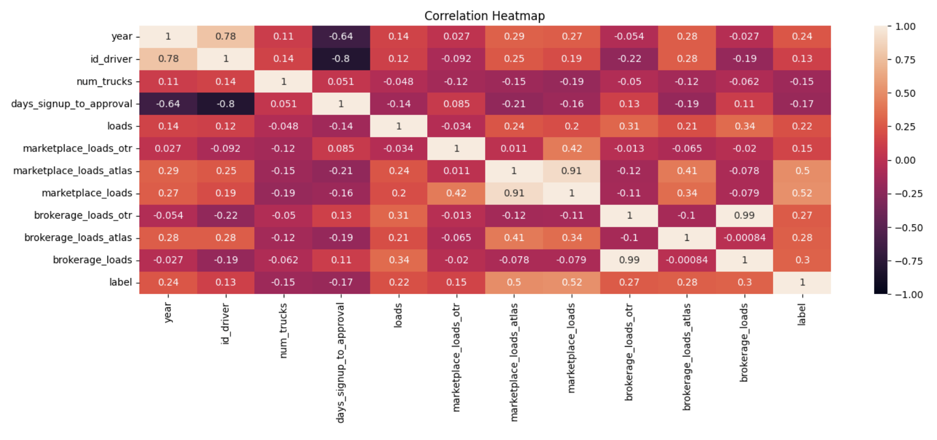
To understand the variable importance of the training dataset, we created the correlation matrix, shown below, to summarize the relationships between the numerical features and the label.
Notable Correlations
The marketplace and brokerage loads features have the strongest positive correlations with high-performing drivers. This does make sense considering we used the total_loads variable to create the label. Within the marketplace loads, drayage type loads have a significantly stronger positive correlation than marketplace over-the-road type loads. This shows us that the more active drivers on the NEXT marketplace platform are those that can perform drayage services. This is a good sign considering we decided to create the can_perform_drayage variable earlier.
The other numerical variables appear to be not as indicative of high-performing drivers. For example, the number of trucks associated with a driver’s carrier is surprisingly negatively correlated with high-performing drivers. I do enjoy looking a visual heatmap and seeing which features correlate and which don’t.
Model Development
Looking at our categorical data, we don’t want features that are too highly correlated. This is because in statistical modeling, the common assumption is that the variables are independent, and there is no inherent correlation between them. Our model needs to be free of redundancy and multicollinearity, which means strong correlation between two features.
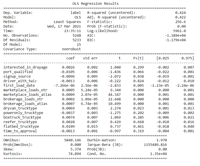
The image above shows our linear regression model.
To better understand the importance of categorical variables, we trained a linear regression model on our manipulated dataset, removing features that contributed to multicollinearity. We don’t want features that are highly correlated, Many variables were correlated in unexpected ways, such as num_trucks and driver_with_twic, so the interpretability of the values in Figure 2 are lessened.
Statistically Significant Features
To know if something is statistically significant, the P-Value has to be less than 0.05. From the results, we see that the following features are statistically significant:
- first_load_date
- marketplace_loads_otr
- marketplace_loads_atlas
- brokerage_loads_otr
- brokerage_loads_atlas
- Dryvan_trucktype
Neural Network Classifier
A neural network classifier was used to create a predictive model. The model employed two hidden layers, with five and two neurons in each respective layer. Each layer used ReLU activation function to avoid a vanishing gradient.
Cross Validation
A 10-fold cross validation was performed on this neural network and on a decision tree ensemble using bagging. The neural network was found to have a mean accuracy of 98.5% in this validation while the bagging ensemble had a 98.8% accuracy.
Cross validation is done to avoid over fitting and poor generalization. Over fitting occurs when the model learns the training data too well, and it fails to generalize well to new data. What cross validation does is simulates the process of
Interpretation
High performing drivers have the strongest correlations with the total number of loads that a driver has delivered, making it a prime indicator for high performance. It may seem that the answer was obvious, but now we have statistics to prove it.
Our neural network created a predictive model that is very accurate, since only 0.97% of the predictions were incorrect. NEXT can run our models to determine which of their drivers are high performing to a fairly high degree of accuracy. They can look for drivers that have high marketplace and brokerage load quantities, which correlate with high performance. It goes without saying that data science is an iterative process, and our work on these classifiers is perhaps only one iteration in the potential lifespan of this project.